1D Array Indices to N-Dimensional Coordinates

If we have values in an \(m\) by \(n\) plane, such that \((m, n) \in \mathbb{R}^2\), we may want to convert the \(x\) and \(y\) coordinates to a single index to store them in a single array within consecutive slots of memory. We can do this using the integer division and modulo functions. We can also generalize this to higher, or \(n\), dimensional tensors.

To keep this simple and build up our explanation, let’s start with a couple of definitions and follow that up with a simple case of converting from \((x, y)\) to an index value and back.

First of all, what’s a tensor? Tensors have been around for a long time, but we hear the term a lot more frequently due to their use in artificial intelligence. We can think of a tensor as an \(n\)-dimensional array. A rank \(0\) tensor is just a scalar value, a number like \(2\) or \(15\), a rank \(1\) tensor is a vector, a rank \(2\) tensor is a matrix, and so forth and so on. So, a tensor is just a generalization of collections of numbers. We can think of the rank as the number of degrees of freedom or axes.

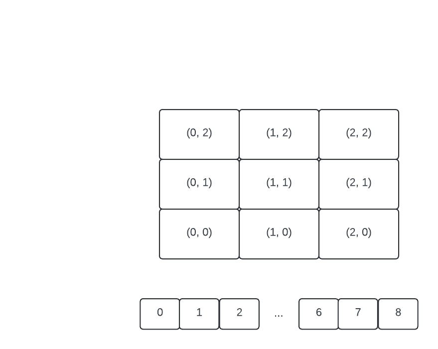
Let’s start off with a \(3\) by \(3\) plane. I’m going to put the origin in the lower left position to have it visually map more naturally to the cartesian plane, but we could have structured it more matrix-like and put the \((0, 0)\) position in the upper left and everything will work out the same. We also have an array with \(9\) empty elements with indices from \(0\) to \(8\).

Using matrix language, we’ll define \(\delta_x\) as the number of columns, \(n\), and \(\delta_y\) as the number of rows, \(m\). Therefore, we have an \(m \times n\) matrix, or \(\delta_y \times \delta_x\) matrix.

We can find the index with the formula,

where \(I\) is the index value.

Before we jump into computations, let’s make a few connections here. If we look at this equation, you may notice that it looks a lot like the equation for a line,

You may also notice that it looks a lot like the equation of integer division with a remainder,

We can keep going and notice that it looks a lot like the modulo equation

which is related to the modulo congruency equation,

which says that \(a - r\) is an integer multiple of \(b\). I know this is a lot, so we’ll unpack it slowly. Let’s start off by computing the indices by hand.

So, how can we find the \(x\) and \(y\) values from the index?

says that \(I - x\) is an integer multiple of \(\delta_x\), or

or x = I % delta_x.

Since I’m directing this post towards programmers, let’s write a little code to frame this a little better. We’ll use Julia since it’s a great language, it’s fast as hell, and it’s super easy to understand.

for idx in 0:8
    @show idx % 3
end

idx % 3 = 0
idx % 3 = 1
idx % 3 = 2
idx % 3 = 0
idx % 3 = 1
idx % 3 = 2
idx % 3 = 0
idx % 3 = 1
idx % 3 = 2

Just like in our hand-derived computations, we can see that for each index value from \(0\) to \(8\), we’re getting \(0\), \(1\), \(2\) cycling. This makes sense because for a \(3 \times 3\) matrix, our \(x\) value will be one of the three.

What about our \(y\) value?

for idx in 0:8
    @show div(idx, 3) % 3
end

div(idx, 3) % 3 = 0
div(idx, 3) % 3 = 0
div(idx, 3) % 3 = 0
div(idx, 3) % 3 = 1
div(idx, 3) % 3 = 1
div(idx, 3) % 3 = 1
div(idx, 3) % 3 = 2
div(idx, 3) % 3 = 2
div(idx, 3) % 3 = 2

Putting these together, lets generate our \(x\) and \(y\) values.

for idx in 0:8
    @show idx
    @show (x, y) = (idx % 3, div(idx, 3) % 3)
end

idx = 0
(x, y) = (idx % 3, div(idx, 3) % 3) = (0, 0)
idx = 1
(x, y) = (idx % 3, div(idx, 3) % 3) = (1, 0)
idx = 2
(x, y) = (idx % 3, div(idx, 3) % 3) = (2, 0)
idx = 3
(x, y) = (idx % 3, div(idx, 3) % 3) = (0, 1)
idx = 4
(x, y) = (idx % 3, div(idx, 3) % 3) = (1, 1)
idx = 5
(x, y) = (idx % 3, div(idx, 3) % 3) = (2, 1)
idx = 6
(x, y) = (idx % 3, div(idx, 3) % 3) = (0, 2)
idx = 7
(x, y) = (idx % 3, div(idx, 3) % 3) = (1, 2)
idx = 8
(x, y) = (idx % 3, div(idx, 3) % 3) = (2, 2)

# Define the dimensions of our matrix where width = cols = delta_x 
# and height = rows = delta_y.
width, height = (3, 3)

# Create a function to compute the index for a R^2 matrix.
function find_r2_index(x::Int, y::Int, dims::Tuple{Int, Int})::Int
    return x + y * dims[2]
end

idx = 5


for idx in 0:8
    x = mod(idx, 3)
    y = mod(div(idx, 3), 3)
    z = div(div(idx, 3), 3)
    @show (x, y, z)
end



(m, n) = (3, 3)
(x, y, z) = (0, 2, 0)
idx = x + y*m + z*m*n

@show idx
@show (x, y, z);