Written by Daniel Marvin
on April 04, 2024

Implementing Norms

Artificial Intelligence (AI) models often need some sort of quantity or length function so we can get a single numeric value from a vector with many components. I actually prefer to think about these as “value” functions, because these functions give us a way to reflect an amount or value, in the economic sense, for any particular vector.

The concept of length is something that only makes sense in lower dimensionality like \(\mathbb{R}\), \(\mathbb{R}^2\), and \(\mathbb{R}^3\). When we start talking about four, five, or \(n\) dimensions, the concept of length no longer has the same meaning. Norms are a generalization of a length function and ultimately are used for computing the length of vectors in an abstract vector space.

This does a few things such as allowing us to compare two vectors numerically – we get a real number from a vector, so we can ask the question: how much?

Let \(V\) be an abstract vector space over a field \(\mathbb{F}\). The norm is a function \(\eta : V \rightarrow \mathbb{R}\), such that,

\(\eta(x + y) \leq \eta(x) + \eta(y)\) for all \(x, y\) in \(V\),
\(\eta(\alpha x) = \vert \alpha \vert \eta(x)\) for all \(x\) in \(V\) and \(\alpha\) in \(\mathbb{F}\), and
for all \(x\) in \(V\), \(\eta(x) = 0\) if and only if \(x = 0\).

The Absolute Value Function

\[\eta(x) = \vert x \vert\]

As an initial example, we’ll discuss the absolute value function. From a programming perspective, it’s simply something which for any scalar value, \(\pm x\), we will always get a positive scalar value.

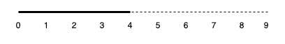
\[\eta(\pm x) = \vert \pm x \vert = x\]

For example, whether we are talking about a vector from the origin to \(-4\) or a vector from the origin to \(4\), the length is still \(4\) in both cases.

Does this satisfy all of the properties of a norm? Let’s verify it with a direct proof, but we’ll use some concrete numbers for a little extra clarity.

Suppose we have two vectors, \(x_1 = 4\) and \(x_2 = -3\) in \(\mathbb{R}\), and let \(\alpha = 2\).

\[\eta(x_1 + x_2) = \eta(4 - 3) = \eta(1) = 1 \leq \eta(4) + \eta(-3) = 4 + 3 = 7\]

Since \(1 \leq 7\), it satisfies the first property. Next, we will check the second.

\[\eta(\alpha x_2) = \alpha \eta(x_2) = 2 \cdot \eta(-3) = 2 \cdot 3 = \eta(2 \cdot -3) = \eta(-6) = 6\]

Finally, since the absolute value function will always return a positive number, the only possible way we can get \(0\) would be if we had a vector \(x = 0\). The absolute value function, abs, satisfies all of the properties of a norm.

The \(\ell^1\) Norm

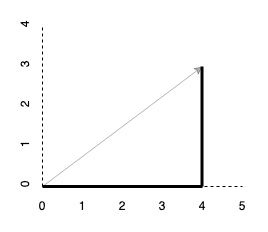
\[\eta(x) = \lVert \mathbf{x} \rVert_1 = \sum_{i=1}^n \vert x_i \vert\]

The \(\ell^1\) norm will trace along the components of the vector rather than calculate the distance along the hypotenuse.

If we have a vector \((4, 3)\) in \(\mathbb{R}^2\), we expect to have a length of \(7\) since \(4 + 3 = 7\).

function l1norm(X::Vector{T})::Real where T<:Real
    [abs(x) for x in X] |> sum
end

The \(\ell^2\) Norm

Instead of adding each of the components, with the \(\ell^2\) norm, we will square each of the components and then take the square root to determine the length of the hypotenuse.

\[\eta(x) = \lVert \mathbf{x} \rVert_2 = \sqrt{x_1^2 + \cdots + x_n^2 }\]

For our \((4, 3)\) vector, this yields a length of \(5\),

\[\sqrt{16 + 9} = \sqrt{25} = 5 \ .\]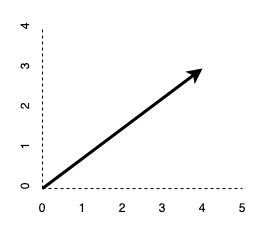

function l2norm(X::Vector{T})::Real where T<:Real
    map(x -> x*x, X) |> sum |> sqrt
end

The \(\ell^p\) Norm

We can generalize this further and account for any variations by implementing the \(\ell^p\) norm.

\[\eta(x) = \lVert \mathbf{x} \rVert_p = \Big( \sum_{i=1}^n \vert x_i \vert^p \Big)^{1/p}\]

The only variation to the \(\ell^p\) norm is when \(p\) approaches infinity. For the \(\ell^\infty\) norm, we define it as,

\[\eta(x) = \lVert \mathbf{x} \rVert_\infty = \max \vert x_i \vert \ .\]

We can therefore represent all \(\ell\) norms with a single function where we vary \(p\) and add a conditional to account for the case when \(p\) approaches infinity.

function lpnorm(X::T; p = 1)::Real where T<:Real
    if isinf(p)
        [abs(x) for x in X] |> maximum
    else
        ([abs(x)^p for x in X] |> sum)^(1/p)
    end
end

@testset "ℓp Norms" begin
    X = [ 4 ; 3 ]
    @test lpnorm(X) == 7.0
    @test lpnorm(X; p=2) == 5.0
    @test lpnorm(X; p=Inf) == 4.0
end

>  Test Summary: | Pass  Total
>  ℓp Norms      |    3      3

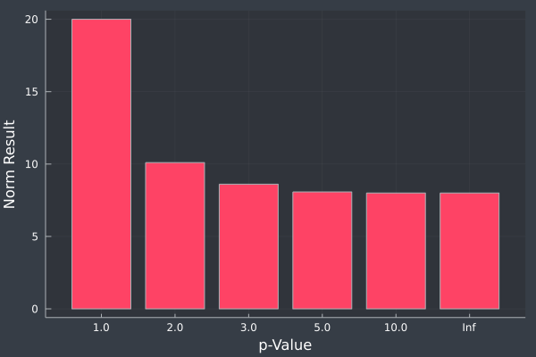
We can plot the result for our \((4, 3)\) vector given different values of \(p\).

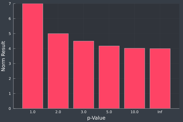
Plotting the same \(p\) values for a \(5\)-dimensional vector, \((4, 3, -2, 3, 8)\), we get the same pattern of smaller length values reducing monotonically as \(p\) increases.

← → Top